Predicting Materials with Artificial Intelligence: A Case Study of the A-Lab and a New Mechanism for Determination of Stable Crystal Structures
It’s one thing to predict the existence of a material, but quite another to actually make it in the lab. That is where the A-Lab fits in. Gerbrand Ceder is an materials scientist at LBNL and the University of California, Berkeley who led the A-Lab team.
Still, it’s clear that systems such as GNoME can make many more computational predictions than even an autonomous lab can keep up with, says Andy Cooper, academic director of the Materials Innovation Factory at the University of Liverpool, UK. Cooper said that computation tells them what to make. A lot more of the predicted material’s chemical and physical properties will have to be calculated by artificial intelligence systems.
Chemists have synthesised many hundred thousand compounds in the lab, though not based on the chains of carbon atoms found in organic chemistry. Yet studies suggest that billions of relatively simple inorganic materials are still waiting to be discovered3. So where to start looking?
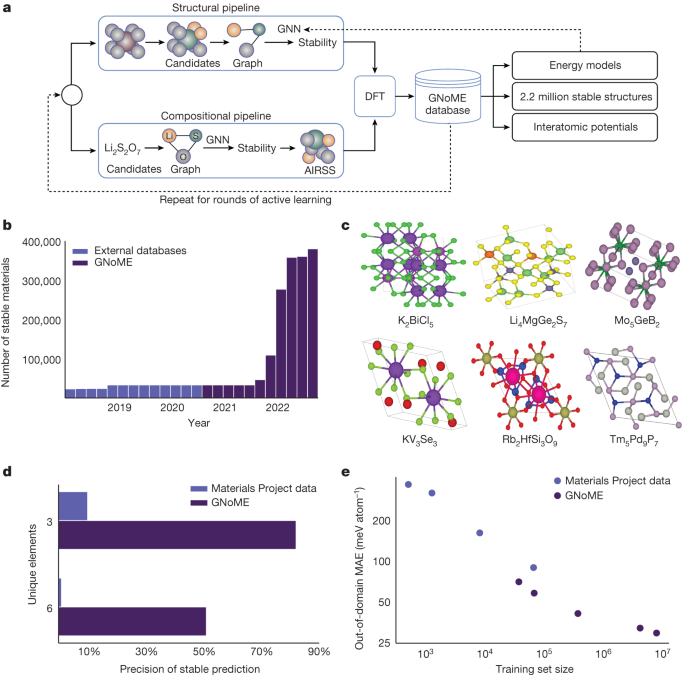
Active learning was performed in stages of generation and later evaluation of filtered materials through DFT. In the first stage, materials from the snapshots of the Materials Project and the OQMD are used to generate candidates with an initial model trained on the Materials Project data, with a mean absolute error of 21 meV atom−1 in formation energy. Filtration and subsequent evaluation with DFT led to discovery rates between 3% and 10%, depending on the threshold used for discovery. New structural GNNs are trained to improve their predictive performance after each round of active learning. Stable crystal structures add to the set of materials that can be replaced and the more candidates are removed from the models. This procedure of retraining and evaluation was completed six times, yielding the total of 381,000 stable crystal discoveries. Continued exploration with active learning may lead to higher stable crystals.
A-Lab: Automated Mixing, Heating and Analyzing for Solid Ingredients Using XtalFinder, a parallel machine learning library
The A-Lab, housed at LBNL, uses state-of-the-art robotics to mix and heat powdered solid ingredients, and then analyses the product to check whether the procedure worked. The US$2-million set-up took 18 months to build. But the biggest challenge lay in using AI to make the system truly autonomous, so that it could plan experiments, interpret data and make decisions about how to improve a synthesis. The innovation is really under the hood, according to Ceder.
We validate the novel discoveries using XtalFinder (ref. 39), using the compare_structures function available from the command line. It was parallelized to 96 cores in order to improve performance. We also note that the symmetry calculations in the built-in library fail on less than ten of the stable materials discovered. There is a low number of failures that suggests a minimal impact on the number of stable prototypes.
“Scientific discovery is the next frontier for AI,” says Carla Gomes, co-director of the Cornell University AI for Science Institute in Ithaca, New York, who was not involved in the research. “That’s why I find this so exciting.”
Reduced Constraint on Oxidation-State-Balanced Composition Models for Structural Substitution
Datamined probabilities are used to make structural substitution patterns. There were 22 events in this event. That work introduced a probabilistic model for assessing the likelihood for ionic species substitution within a single crystal structure. Calculating the probability of substitution is done by using a binaries feature model. The model is simplified so that fi is 0 or 1 if a specific substitution pair occurs and λi provides a weighting for the likelihood of a given substitution. The resulting probabilities have aided in discovering new quaternary imoniac compounds.
For the compositional pipeline, inputs for evaluation by machine-learning models must be unique stoichiometric ratios between elements. Enumerating the combinatorial number of reduced formulas was found to be too inefficient, but common strategies to reduce such as oxidation-state balancing was also too restrictive, for example, not allowing for the discovery of Li15Si4. In the paper, we introduce a relaxed constraint on oxidation-state balancing. We start with the common oxidation states of the Semiconducting Materials by Analogy and Chemical Theory, with 0 for metallic forms. Between two oxidation states, we can allow up to two elements to exist. Although this is a heuristic approach, it substantially improves the flexibility of composition generation around oxidation-state-balanced ratios.
For the models, each element in the composition is represented by a Node so that they are as efficient as possible. The ratio of the element is compared to the one-hotvector. For example, SiO2 would be represented with two nodes, in which one node feature is a vector of zeros and a 1/3 on the 14th row to represent silicon and the other node is a vector of zeros with a 2/3 on the 8th row to represent oxygen. Although this simplified GNN architecture is able to achieve state-of-the-art generalization on the Materials Project (MAE of 60 meV atom−1 The predictions for materials discovery do not offer anything useful. One of the issues with compositional models is that they assume that the training label refers to the ground-state phase of a composition, which is not guaranteed for any dataset. Thus, the formation-energy labels in the training and test sets are inherently noisy, and reducing the test error does not necessarily imply that one is learning a better formation-energy predictor. To explore this, we created our own training set of compositional energies, by running AIRSS simulations on novel compositions. Compositions with only a few completed AIRSS runs tend to have larger formation energies than predicted, according to supplementary note 5. We find that if we limit ourselves to compositions for which at least 10 runs are completed, the GNN error is reduced to 40 meV atom1. We then use the GNN trained on such a dataset (for which labels come from the minimum formation energy phase for compositions with at least ten completed AIRSS runs and ignoring the Materials Project data) and are able to increase the precision of stable prediction to 33%.
As we describe in Supplementary Note 5, not all DFT relaxations converge for the 100 initializations per composition. A few of the initializations converge for certain compositions. A good initial volume guess for the composition is one of the main difficulties. We try a range of initial volumes ranging from 0.4 to 1.2 times a volume estimated by considering relevant atomic radii, finding that the DFT relaxation fails or does not converge for the whole range for each composition. Prospective analysis was not able to uncover why most AIRSS initializations fail for certain compositions, and future work is needed in this direction.
We train on formation energies instead of total energies. Formation energies and forces are not normalized for training but instead we predict the energy as a sum over scaled and shifted atomic energies, such that (\widehat{E}={\sum }{i\in {N}{{\rm{atoms}}}}\left({\widehat{{\epsilon }}}{i}\sigma +\mu \right)), in which ({\widehat{{\epsilon }}}{i}) is the final, scalar node feature on atom i and σ and μ are the standard deviation and mean of the per-atom energy computed over a single pass of the full dataset. The network was trained on a joint loss function consisting of a weighted sum of a Huber loss on energies and forces:
Following Roost (representation learning from stoichiometry)58, we find GNNs to be effective at predicting the formation energy of a composition and structure.
Discovering new datasets aided by neural networks requires a careful balance between ensuring that the neural networks trained on the dataset are stable and promoting new discoveries. New structures and prototypes will be inherently out of distribution for models; however, we hope that the models are still capable of extrapolating and yielding reasonable predictions. The implicit domain shift, in which models are evaluated before relaxation, is contributing to the out-of-distribution detection problem. These effects were counteracted through several adjustments to test-time predictions.
Augmentations at test time are often used to correct machine- learning predictions. We consider the isotropic scaling of the lattice vectors for specific structural models. Minimum reduction is used to aggregate at 20 values ranging from 80% to120% of the reference lattice scaling volume. This has the added benefit of potentially correcting for predicting on nonrelaxed structures, as isotropic scaling may yield a more appropriate final structure.
Although neural network models offer flexibility that allows them to achieve state-of-the-art performance on a wide range of problems, they may not generalize to data outside the training distribution. The use of models in an ensemble is a simple choice for improving machine-learning predictions. Training n models is what it takes to use this technique. The prediction is related to the mean over the outputs of all the models, and the uncertainty can be measured by the spread of the outputs. We use 10 graph networks to train machine- learning models for stability prediction. Moreover, owing to the instability of graph-network predictions, we find the median to be a more reliable predictor of performance and use the interquartile range to bound uncertainty.
Source: Scaling deep learning for materials discovery
Automated Quantification of Stable Materials Using the VASP and r2SCAN for Active-Learning Simulations and DFT Verification
For active-learning setups, only the structure predicted to have the minimum energy within a composition is used for DFT verification. For an in-depth evaluation of a particular family, we design clustering-based reduction strategies. We compare the top 100 structures to pymatgen’s built-in structure matcher and take a look at any given composition. The minimum energy structure is used to represent the cluster on the graph of pairwise similarities. This provides a scalable strategy to discovering polymorphs when applicable.
We use the VASP with both PBE41 functional and PAW40,60 potentials in DFT calculations. The settings in the DFT are consistent with the Materials Project. The settings for the Materials Project include Hubbard U, 520 eV plane-wave-basis cutoff, magnetization, and the choice of PBE pseudopotentials. For Li, Na, Na, Mg, Ge, and Ga we use newer versions of their potentials with the same number of electrons. For all structures, we use the standard protocol of two-stage relaxation of all geometric degrees of freedom, followed by a final static calculation, along with the custodian package23 to handle any VASP-related errors that arise and adjust appropriate simulations. The more traditional Monkhorst–Pack doesn’t force gamma centred k point generation for hexagonal cells. Computational costs for different spin orderings were prohibitive at the scale presented, and we assume ferromagnetic spin initialization with finite magnetic moments. The AIMD simulations use the NVT ensemble with a 2-fs time step.
For validation purposes (such as the filtration of Li-ion conductors), bandgaps are calculated for most of the stable materials discovered. We automate bandgap jobs in our computation pipelines by first copying all outputs from static calculations and using the pymatgen-based MPNonSCFSet in line mode to compute the bandgap and density of states of all materials. A full analysis of patterns in bandgaps of the novel discoveries is a promising avenue for future work.
r2SCAN is a functional that has seen increased adoption from the community for increased fidelity in computational DFT calculations. The settings for this function are provided by the upgraded version of VASP6 and we also use them for all corresponding calculations. Notably, r2SCAN functionals require the use of PBE52 or PBE54 potentials, which can differ slightly from the PBE equivalents used elsewhere in this paper. To speed up computation, we perform three jobs for every SCAN-based computation. We need to precondition by using the PBE54 potentials by running a standard relaxation job. The preconditioning step speeds up SCAN computations, which are five times slower, and can cause crashes in our infrastructure. Then, we relax with the r2SCAN functional, followed by a static computation.
The materials project and the O QMD has the same DFT settings as pymatgen allows us to change them in a consistent way to calculate the total number of stable crystals. Furthermore, to ensure fair comparison and that our discoveries are not affected by optimization failures in these high-throughput recalculations, we use the minimum energy of the Materials Project calculation and our recalculation when both are available.
To count the number of layered materials, we use the methodology developed in ref. 45, which is made available through the pymatgen.analysis.dimensionality package with a default tolerance of 0.45 Å.
Source: Scaling deep learning for materials discovery
High-Throughput Determination of the Li/Mn Transition Metal Oxide Conductor Number in Superconducting Graph Networks
The estimated number of viable Li-ion conductors reported in the main part of this paper is derived using the methodology in ref. 46 in a high-throughput fashion. This methodology involves applying filters based on bandgaps and stabilities against the cathode Li-metal anode to identify the most viable Li-ion conductors.
The Li/Mn transition metal oxide family is discussed in the ref. To look at the capabilities of machine-learning models. The main text has a comparison against the findings of the work with previous machine- learning methods.
To allow a fair comparison with the smaller M3GNet dataset used in ref. 62, a NequIP model was trained on the M3GNet dataset. We chose the hyperparameters in a way that balances accuracy and computational efficiency, resulting in a potential with efficient inference. We train in two setups, one splitting the training and testing sets based on unique materials and the other over all structures. In both cases, we found the NequIP potential to perform better than the M3GNet models trained with energies and forces (M3GNet-EF) reported in ref. 62. The NequIP model was trained on structure-split M3GNet data and is used for zero-shot comparisons in the scaling tests. We expect our scaling and zero-shot results to be applicable to a wide variety of modern deep-learning interatomic potentials.
JAX and capabilities to just-in-timecompile programs onto devices such as graphics processing units and tensor processing units make use of GNoME models for machine learning. Graph networks implementations are based on the framework developed in Jraph, which makes use of a fundamental GraphsTuple object (encoding nodes and edges, along with sender and receiver information for message-passing steps). JAX MD is written for processing crystal structures as well as TensorFlow for parallelized data input64.
Large-scale generation, evaluation and summarization pipelines make use of Apache Beam to distribute processing across a large number of workers and scale to the sizes as described in the main part of this paper (see ‘Overview of generation and filtration’ section). Billions of proposal structures require extra storage that wouldn’t otherwise fail on single nodes.
Source: Scaling deep learning for materials discovery
Out-of-Distribution Robustness Test of NequIP and Fine-Pitchted Models on Artificial Intelligence Data
The training set sizes for the models were increased from 400 to 600 for testing the robustness. We then evaluate these models on AIMD data sampled at both T = 400 K (to measure the effect of fine-tuning on data from the target distribution) and T = 1,000 K (to measure the robustness of the learned potentials). A NequIP model was pretrained before the learning rate was reduced, and a fine-pitched model was trained at the checkpoint before the learning rate was reduced. The network architecture is identical to that used in pretraining. Because the AIMD data contain fewer high-force/high-energy configurations, we use a L2 loss in the joint loss function instead of a Huber loss, again with λE = 1.0 and λF = 0.05. For all training set sizes and all materials, we scan learning rates 1 × 10⁻² and 2 × 10⁻³ and batch sizes 1 and 16. Models are trained for a maximum of 1,000 epochs. If the test error on a hold-out set was not better for 50 epochs, the learning rate is reduced by 0.8. We choose the best of these hyperparameters based on the performance of the final checkpoint on the 400-K test set. The 400-K test set is created using the final part of the AIMD trajectory. Sampling different set sizes from the initial part of the AIMD trajectory is what creates the training sets. The out-of-distribution robustness test is generated from the AIMD trajectory at 1,000 K. Training is performed on a single V100 GPU.
$${\mathcal{L}}={\lambda }{E}\frac{1}{{N}{{\rm{b}}}}\mathop{\sum }\limits_{b=1}^{b={N}{{\rm{b}}}}{{\mathcal{L}}}{{\rm{Huber}}}\left({\delta }{E},\frac{{\widehat{E}}{{\rm{b}}}}{{N}{{\rm{a}}}},\frac{{E}{{\rm{b}}}}{{N}{{\rm{a}}}}\right)+{\lambda }{F}\frac{1}{{N}{{\rm{b}}}}\mathop{\sum }\limits{b=1}^{b={N}{{\rm{b}}}}\mathop{\sum }\limits{a=1}^{b={N}{{\rm{a}}}}{{\mathcal{L}}}{{\rm{Huber}}}\left({\delta }{F},-\frac{\partial \widehat{{E}{{\rm{b}}}}}{\partial {r}{{\rm{b}},{\rm{a}},\alpha }},{F}{b,a,\alpha }\right)$$
The structural model was trained using the Adam optimizer, which has a learning rate of 2 103 and a processing size of 16. The learning rate was decreased to 2 × 10⁻⁴ after 601 epochs, after which we trained for another 200 epochs. We use the same joint loss function as before in the training that we did, again with E, F and E. The network hyperparameters are identical to the NequIP model used in GNoME pretraining. To enable a comparison with ref. 62, we also subtract a linear compositional fit based on the training energies from the reference energies before training. Training was performed on a set of four V100 GPUs.
Source: Scaling deep learning for materials discovery
Classification of superionic materials by their conductivities and Diffusion Analyzer with the Anti-Ionized Gas Detector (AIMD)
Following ref. 69, we classify a material as having superionic behaviour if the conductivity σ at the temperature of 1,000 K, as measured by AIMD, satisfies σ1,000K > 101.18 mScm−1. Refer to the original paper for applicable calculations. Supplementary information can be found for further details.
The materials for AIMD simulation are chosen solely on the basis of factors such as stability, chemistry and band gap. The search for electrolytes should not include materials with notable electronic conductivities, that is the last criterion. Materials are run in their pristine structure, that is, without vacancies or stuffing. The AIMD simulations were done with the VASP. The temperature isinitialized at 300 K and then increased over a time span of 5 ps to the target temperature. This is followed by a 45-ps simulation equilibration using a Nosé–Hoover thermostat in the NVT ensemble. Simulations are done at a 2-fs time step.
The first 10 ps of the machine learning simulation are discarded for equilibration for analysis of the AIMD. From the final 40 ps, we compute the diffusivity using the DiffusionAnalyzer class of pymatgen with the default smoothed=max setting23,70,71.