A dataset of serial-section electron microscopy images from a female mouse with radial extent of dendritic arbour

This dataset is composed of 1.1mm 800 m and 600 m segments of a serial-section electron microscopy dataset from a male mouse. The dataset covers both the primary and higher visual areas of the cortex. The data has been described in detail. Briefly, two-photon imaging was carried out on the mouse, which was subsequently prepared for electron microscopy. The specimen was then sectioned and imaged using transmission electron microscopy6. The images were then stitched, aligned and processed through a deep learning segmentation algorithm, followed by manual proofreading5,6,7,15.

The column borders were found using a method that identifies a region from the primary visual cortex far away from both the boundaries and the higher-order visual areas. The box was placed along the axis of the dataset on the basis of layer 2.

Radial extent of dendritic arbour. We define ‘radial distance’ to be the distance in the same plane as the pial surface. For every neuron, we computed a pia-to-white-matter line, including slanted region in deep layers, passing through its cell body. For each skeleton vertex, we computed the radial distance to the pia-to-white-matter line at the same depth. To avoid any outliers, the radial extent of the neuron was defined to be the 97th percentile distance across all vertices.

By looking at all the branch points, we began cleaning the axons of false merges. We then performed extension of axonal tips until either their biological completion or data ambiguities, particularly emphasizing all thick branches or tips that were well-suited to project to new laminar regions. For axons with many thousands of synaptic outputs, we followed many but not all tips to completion once primary branches were cleaned and established. Some tips were extended to the point of completion or ambiguity, for smaller neurons. The amount of axon length and the thickness of it affect the quality of autosegmentations, and in turn the amount of axon time. In the past, axon cleaning and extension took a minimum of 3 h per neuron.

We defined an object as the segmentation associated with a predicted nucleus5 from which nucleus, soma and PSS features could be extracted. A hierarchical framework was designed to predict the cell type of any such object (Fig. 5c). There are over 100,000 nuclear segments that passed the first two filters described in the section entitled Filtering procedure. The first level of the hierarchy predicted an object’s structure, whether a neuron or a non-neuron, and an error. All objects predicted as errors were excluded from all subsequent analyses except for the hierarchical model evaluation. In order to classify non-neuronal cells they were grouped into three categories:Astrocyte (7,850), microglia (2,663), and oligodendrocytes (7,020). Cells were predicted either as excitatory (64,195) or conjugate (7,962) with a separate subclass classification for each class type. Excitatory subclasses were layer 2/3 pyramidal (19,735), layer 4 pyramidal (14,777), layer 5 IT (7,949), layer 5 ET (2,215), layer 5 near-projecting (NP) pyramidal (970), layer 6 IT (11,734) and layer 6 CT pyramidal (6,815). After extracting PSS features from all predicted inhibitory neurons, a subset of neurons (n = 1,158) that were actually excitatory clearly separated from the rest of the cells in the perisomatic feature space (with PSS features). This was expected owing to known differences in proximal dendrite morphology between inhibitory and excitatory neurons. The total number of cells in the excitatory neuron classification was 6,796, with 3,239 basket cells and 97 Martinotti/non-Martinotti cells.

Nucleus Prediction Map from the MICrONS Dataset: The Distributions of Connections and Synapses in each Subclass

The training set was changed with manually labelled errors from the entire dataset due to the fact that there were few errors in the column.

Median radius across dendritic skeleton vertices. To avoid the region immediately around the soma from having a potential outlier effect, we only considered skeleton vertices at least 30 µm from the soma.

A computer trained to predict if a voxel was in a cell nucleus. Following the methods described in ref. 69, a nucleus prediction map was produced on the entire dataset at 64 × 64 × 40 nm3.

To measure the predicted cell densities per subclass across the MICrONS dataset, we divided the dataset into 50-µm2 bins in the x–z plane. To make comparisons between reported densities in the literature and the actual number of cells in each bin, we scaled the number of cells in each subclass to the number per square millimetre.

We fit a simple model to match the numbers of connections and the number of synapses in the distribution. We used a chi-squared test to probe whether the measured distributions were significantly different from the Poisson model. For each cell, the total number and distribution of output spees onto it were calculated. We calculated the number of single-, double- and triple-synapse (up to 17-synapse) containing connections for each presynaptic MC onto each target cell type (L2/3, L4, L5 ET, and so on), then built a Poisson distribution for each presynaptic cell and postsynaptic target cell type using the total number of connections and the average number of synapses per connection. We used a chi-squared test to compare the real and Poisson distributions, and found that the null hypothesis about the distributions being the same could not be rejected.

Soma and nucleus features were extracted from the 3D mesh of all objects and PSS features were extracted for all neurons predicted as inhibitory. For each level of the hierarchy, multiple classifiers were trained using either nucleus alone, nucleus and soma features, or nucleus, soma and PSS features. The cortical column was used to train the classes within the hierarchy. Owing to the sparsity of some of the cell classes, we augmented the training set in the following ways: 470 errors were added from within and around the column for the object model; 11 proofread 5P-NP cells and 250 proofread 5P-ET cells were added to train the excitatory subclass model.

The top level of the hierarchy distinguishes between neurons from non-neurons and incorrect detections. The accuracy score on the column was cross-validated using a test score of 97%. The second level of the model simply distinguished excitatory from inhibitory neurons. Here, the column cross-validated accuracy score was 94% and the test set was 93%. Overall, across all subclasses, the hierarchical model on the column had a cross-validated accuracy of 91% and a dataset-wide test set accuracy of 82%.

The model types were chosen based on a randomized grid search for the following: support vectors machine with a linear kernels, supportvector machine with a radial function kernel, nearest neighbours, random forest and neural network. For each type, 50 models were trained with varying parameters and the top-performing model was chosen. Individual models were further optimized using tenfold cross-validation evaluated on the basis of accuracy and F1 score (a measure for precision and recall). Training and test examples were held the same across models.

Clustering excitatory neurons on the basis of ten nearest-neighbourhood graphs and application to 2D UMAP training

This collection of features allowed us to cluster excitatory Neurons by running phenograph 77 500 times with the majority of cells included each time. A nearest-neighbourhood graph can be found by using the Leiden to find community on the graph. Here we used a graph on the basis of ten nearest neighbours and clustered with a resolution parameter of 1.3. These values were chosen to consistently separate layer 5 ET, IT and NP cells from one another, a well-established biological distinction. A coclustering matrix was assembled with each element corresponding to the number of times two cells were placed in the same cluster. To compute the final consensus clusters, we performed agglomerative clustering with complete linkage on the basis of the coclustering matrix, with the target number of clusters set by a minimum Davies–Bouldin score and a maximum Silhouette score. Clusters were then named on the basis of the most frequent manually defined cell type in the cluster and reordered on the basis of median soma depth. The cells were classified into two layers, layer 2 and layer 3, on the basis of Soma depth and a flat structure, with no apical trunk or branches in contact with the cell body. The L2c subclass was ambiguously defined between the two categories, with cells that had a distinct apical trunk but with connectivity and other properties that seemed more similar to layer 2 subclasses.

Compartment labels were propagated to synapses on the basis of the associated skeleton vertices. Soma synapses were all those associated with level 2 chunks in the soma collapse region (see the section ‘Skeletonization’). Proximal dendrites were those outside of the soma but within 50 µm after the start of the branch. There weren’t any of them on apical branch because they were more distant than the threshold. Apical junctions were associated with more distant points than the threshold and apical branches.

It was important that all features were placed roughly in the same scales for 2D UMAP training. We used the feature scores from all the cells to give us input for training the classifier and UMAP embedded in the Figs. 3–6.

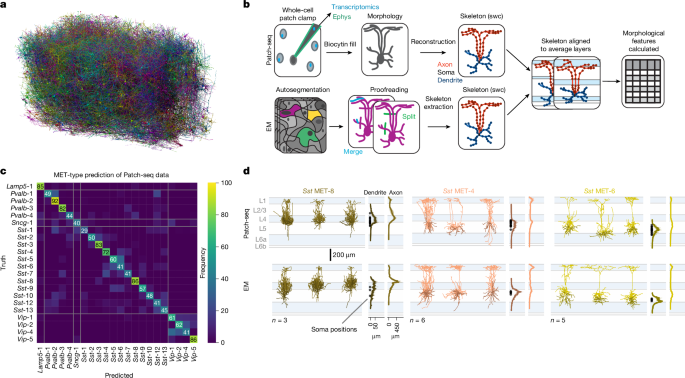
Post hoc comparison of MET-types using the MERFISH data for the cortex and the Myh8 Etv1 and Sst Hpse Cbln4

The Kruskal–Wallis and Conover post hoc tests were used to compare several MET-types. The Kruskal–Wallis P values are indicated on the plots if they are 0.05 or P 0.01. Errors reported are s.e.m. unless otherwise indicated. The fraction of cell types targeted by a MET type were compared using a non-P value test, and the false discovery rate was also used. The maximum and minimum range of the data is shown in the boxplot whiskers. Measurements are taken repeatedly from these cells.

We analysed differentially expressed genes using scrattch.hicat to compare the main transcriptomic types. Sst Hpse Cbln4; MET-4 Sst Calb2 Necab1and The Sst Calb2 Pdlim5 is called. MET-6: Sst Chrna2 Glra3, Sst Chrna2 Ptdg4 and Sst Myh8 Etv1). Pairwise differentially expressed genes were identified as previously described6 using the limma package69 and selecting genes with at least a twofold change in expression and an adjusted P value of less than 0.01. The top five upregulated and down regulated genes were ranked by adjusted P value for visualization. The average expression of these genes and the fraction of cells with non-zero expression was calculated for the neurons of the three Sst MET-types in the Patch-seq data16 and presented as a dot plot. Only genes that were expressed in at least half of the cells in the MET type were selected for visualization.

Proportions of MET-types were estimated from a recently published MERFISH dataset67. Cell counts were calculated for each Sst t-type in VISp in the MERFISH dataset. As the cells in the MERFISH dataset were mapped to a whole-brain taxonomy67, whereas the MET-types were based on a VISp-specific taxonomy6, we identified correspondences between t-types across several taxonomies. Correspondences between the original taxonomy of Tasic et al.6 and the cortex or hippocampal formation (CTX/HPF) taxonomy were identified by finding the Tasic et al.6 t-types that had the highest number of shared cells for each CTX/HPF t-type68. Correspondences between the CTX/HPF and whole-brain taxonomy were taken directly from ref. 67. We assigned Tasic et al.6 t-types to the MET-types to which the largest number of cells belonged16, except for the t-type Sst Calb2 Pdlim5, for which corresponding cells were assigned to either Sst MET-3 (if located in L4 or above) or Sst MET-4 (if located in L2/3). Cells from the Sst Chodl subclass were not analysed here. The original study16 contained a small number of cells, and no clear t-type correspondences were found for the MET-type Sst MET-11.

Using automatically detected synapses, annotators visualized all output synapses on a given presynaptic cell in Neuroglancer. Regions lacking synapses were manually inspected in the EM imagery. If myelination was seen, an annotator marked the start and end point of each myelinated segment in Neuroglancer to generate a line. The number of myelinated segments was determined by summing the number of annotations. The distance of myelinated axon to a cell is determined by the length of the annotations.

Cell subclass identities were assigned to all meshes with single somas (individual cells) in the EM dataset using a support vector machine classifier trained on somatic and nuclear features60. This classifier was then applied across the EM dataset to generate predicted cell type identities for most cells. We use these assigned types in all plots shown above. There was broad agreement between the automated and manual methods but there was a disagreement over the identity of targets of the predicted MET-8 cell type. 5b. Labels shown in the figures are from automated assignment.

The mean and s.d. of the data from Patch-seq was used to calculate the Z scores for the features.

A reliability metric was calculated as the fraction of iteration each sample was predicted as its final MET assignment, for example, a cell was predicted 80% of the time. To determine an appropriate threshold, we explored reliability scores in the Patch-seq data. We applied random subsampling in a leave-one-out manner. Here we set one Patch-seq sample aside and use the rest as training data. The training data is sub-sampled randomly for each iteration and used to fit a new code. The classifier predicts the MET-type label of the single left-out Patch-seq sample. This process was repeated 500 times for every Patch-seq cell until each had a predicted MET-type label and corresponding reliability metric. We then plotted a cumulative histogram of the correctly and incorrectly predicted labels versus the reliability score. We found that a reliability score of more than 0.54 is the most inclusive value at which Patch-seq samples are more frequently predicted correctly than incorrectly (Extended Data Fig. 2b.

An RFC, support vector machine and logistic regression model were assessed for performance in predicting MET-type labels for Patch-seq cells using the morphological features of inhibitory cell types from a previously published Patch-seq dataset (Patch-seq n = 477, Sst n = 236, Pvalb n = 89, Vip n = 79, Lamp5 n = 44, Sncg n = 29)16. We used a fivefold cross-validation approach to assess classification accuracy. The data were split randomly into five partitions while maintaining the distribution of MET-type labels in each partition. This method iteratively rotates which partition is withheld from training and used to validate the model. MET-types with fewer than five morphological reconstructions (Lamp5 MET-2, Pvalb MET-5, Sncg MET-2, Sncg MET-3, Sst MET-11 and Vip MET-3) were omitted. An RFC with 250 estimators, a maximum depth of ten, balanced class weights, a minimum of ten samples per split and at least five samples per leaf node outperformed logistic regression and support vector machine models. A mean accuracy of 58.9 4.1% was achieved when fivefold cross-validation was repeated 20 times, far exceeding the expected chance accuracy for 22 categories. The model’s accuracy was determined by how frequently it predicted the MET- type label of held out data. 5b). The F1 score was calculated by dividing the average F1 scores for each type by the total number of MET-types. There was a cumulative confusion matrix for hold- out validation data. 1c.

Meshes underwent skeletonization (skeleton originated from a defined soma point) to generate a list of branch and end points for each mesh, visible in Neuroglancer33. Each branch point was inspected manually. True branch points were left alone and false branch points (often due to overlapping processes from distinct cells) were split using Neuroglancer tools. Subsequently, each end point was inspected manually. True endpoints were left alone and false endpoints (premature end of a process) were extended by an expert annotator, who would follow the process along the EM imagery to a natural ending (bouton, tapered end) or until the process could no longer be extended reliably (for example, edge of block). The total number of EM reconstructions of inhibitory cells used in this study is 173 (including clean and comprehensive reconstructions).

To measure intracolumnar inhibitory connectivity, we first restricted synaptic outputs to the axon of each inhibitory neuron, as we have not observed any correctly classified synaptic outputs on dendritic arbours in this dataset. There was a cell which had less than 30 synaptic outputs. The remaining outputs from all interneurons were then divided in to two categories, with the first one going to the cells in the column. Each output synapse was also labelled with the target skeleton vertex, dendritic compartment and M-type of the target neuron on the basis of the compartment definitions above.

The fraction of multisynaptic connection synapses that were also within 15 µm of another synapse with the same target, as measured between skeleton nodes. Note that we evaluated the robustness of this parameter and found that intersynapse distances from 5 to more than 100 µm have qualitatively similar results (Extended Data Fig. 2).

Using these six features, we trained a linear discriminant classifier on cells with manual annotations and applied it to all inhibitory cells. The differences from manual annotations were seen as a different view of the data.

The median linear density of synapses in an inhibitory molecular input cluster and a connectomic census of mouse visual cortex

Median tortuosity of the path from branch tips to soma per cell. trouosity is the ratio of path length to the distance from tip to soma centroid.

Median linear density of synapses. This was measured by computing the net path length and number of synapses along 50 depth bins from layer 1 to white matter and computing the median. A linear density was found by dividing the sphinx count by the path length per bin and the median was found across all bins.

The features were computed after a rigid rotation of 5 degrees to flatten the pial surface and set the pial surface to 0 on the y axis. Features on the basis of apical classification were not explicitly used to avoid ambiguities on the basis of both biology and classification.

To calculate the importance of each feature, we used a random forest classification to see if a cell belonged to it. Because the classes were strongly imbalanced, we used SMOTE resampling to oversample datapoints from the smaller class. Mean Decrease in Impurity is a metric that shows how often a feature was used in the decision tree ensemble.

For the inhibitory motif group clustering, for each interneuron we first computed the number of synapses across each excitatory M-types in the column. This synaptic output budget was then normalized per cell to generate a vector for each neuron with elements ranging from zero to one. Normalized synaptic output budgets were oversegmented using k-means (k = 20) with Euclidean distances 500 times, and a matrix of coclustering frequency—that is, the number of times two cells were put in the same k-means cluster—between individual cells was computed. A final value of 18 was selected from the scores of two to 25 output clusters, a silhouette score and a Davies–Bouldin score, and through agglomerative clustering.

Source: Inhibitory specificity from a connectomic census of mouse visual cortex

Alignment of an AutoTEM Volume Dataset using a Synaptic Cleft Prediction Network and a Convolutional Network to Predict a Velocities Prediction

On connectivity cards, we also show a similar selectivity index on the basis of compartment rather than M-type. In that case, the shuffled distribution preserves observed depth and M-type output distributions but not compartments.

For synapse detection and assignment, a convolutional network was trained to predict whether a given voxel participated in a synaptic cleft. Inference on the entire dataset was processed using the methods described in ref. 69 using 8 × 8 × 40 nm3 images. These synaptic cleft predictions were segmented using connected components, and components smaller than 40 voxels were removed. A separate network was trained to perform synaptic partner assignment by predicting the voxels of the synaptic partners given the synaptic cleft as an attentional signal72. This assignment network was run for each detected cleft, and coordinates of both the presynaptic and postsynaptic partner predictions were logged along with each cleft prediction.

The curvature is not aligned to a sectioning plane or associated with shearing or other distortion in the imagery, making it unlikely to be a result of the alignment process.

The blood vessel segment doesn’t show a big distortion in deep layers, which is unlikely to be the result of stress on the tissue. It’s not known why stress would only affect layer 5b and below.

Similar curvature has been observed in other large EM datasets from visual cortex (data not shown) and light level morphological reconstructions, particularly among layer 6 pyramidal cells.

The volume assembly is described in detail. The images collected by the autoTEMs are first corrected for lens distortion effects by using a set of 10 10 highly intersecting images. Overlapping image pairs are identified in each section, and point correspondences are extracted using features extracted using the scale-invariant feature transform. Montage transformation parameters are estimated per image to minimize the sum of squared distances between the point correspondences between these tile images, with regularization. The down sample version of these sections was used to estimate the per-section transformation that roughly aligned these sections in three dimensions. For further alignment, the volume is rendered to the disk. The AllenInstitute has a software tool available that is used to align a dataset. The image processing pipeline had to be strong to image and sample artefacts to align the volume. Cracks larger than 30 um (in 34 sections) were corrected by manually defining transforms. The smaller cracks and folds were automatically identified by using a network of networks trained on 64 64 40 nm3 images. The voxels were identified with tissue. The rough alignment was iteratively refined in a coarse-to-fine hierarchy66 using an approach based on a convolutional network to estimate displacements between a pair of images67. Displacement fields were calculated between pairs of sections to produce a final field for each image. First, alignment was refined with 64 64 40 nm3 images and then with 1,024 1,064 40 nm3 images. The composite image of the partial sections was created using the tissue mask previously computed.

The parallel imaging pipeline used in this study61 used a fleet of transmission electron microscopes that had been converted to continuous automated operation. The standard JEOL 1200EX II transmission electron microscope was modified with custom hardware and software for it, and includes a scintillator. A single large-format camera with a low-distortion lens used to grab image frames at 100 ms. The sample stage that was built into the autoTEM offered high-fidelity montaging of tissue sections and a reel- to-reel tape translation system that could locate each section using index barcodes. During imaging, the reel-to-reel GridStage moved the tape and located the targeting aperture through its barcode and acquired a 2D montage. Quality control was done on image data that was failed by screening.

After optical imaging at Baylor College of Medicine, candidate mice were shipped via overnight air freight to the Allen Institute. Mice were transcardially perfused with a fixative mixture of 2.5% paraformaldehyde, 1.25% glutaraldehyde and 2 mM calcium chloride, in 0.08 M sodium cacodylate buffer, pH 7.4. A thick slice was cut and post- fixed for a period of 12–48 h. The slices were prepared and washed for the reduced osmium treatment. 64. Unless stated otherwise, all steps were done at room temperature. The first osmication step involved 2% osmium tetroxide (78 mM) with 8% v/v formamide (1.77 M) in 0.1 M sodium cacodylate buffer, pH 7.4, for 180 min. Potassium ferricyanide 2.5% (76 mM) in 0.1 M sodium cacodylate, 90 min, was then used to reduce the osmium. The second osmium step was at a concentration of 2% in 0.1 M sodium cacodylate for 150 min. Samples were washed with water and then immersed in thiocarbohydrazide for further intensification of the staining (1% thiocarbohydrazide (94 mM) in water, 40 °C, for 50 min). After washing the sample were put in a 2% of water for 90 minutes. After extensive washing in water, Walton’s lead aspartate (20 mM lead nitrate in 30 mM aspartate buffer, pH 5.5, 50 °C, 120 min) was used to enhance contrast. After two rounds of water wash steps, samples proceeded through a graded ethanol dehydration series (50%, 70%, 90% w/v in water, 30 min each at 4 °C, then 3 × 100%, 30 min each at room temperature). Two rounds of acetonitrile (30 min) were used as a transitional solvent step before moving on to the next step. Invade a progressive series that starts with 2:1 and 1 100% acetonitrile. Epoxy was cured at 60 °C for 96 h before unmoulding and mounting on microtome sample stubs. The sections were collected from six reels of grid tape and put onto a modified ATUMtome.

All animal procedures were approved by the Allen Institute for Brain Science and the Waco College of Medicine. Neurophysiology data acquisition was conducted at Baylor College of Medicine before EM imaging. Afterwards the mice were transferred to the Allen Institute in Seattle and kept in a quarantine facility for 1–3 days, after which they were euthanized and perfused. The results described are from a single male mouse who was 64 days old at the start of the experiment. Two-photon functional imaging took place between P75 and P80 followed by two-photon structural imaging of cell bodies and blood vessels at P80. The mouse was perfused at P87.

Source: Inhibitory specificity from a connectomic census of mouse visual cortex

Data acquisition, aligning and segmentation for the MICrONS experiment on atomic nuclei with gravitational neutrinos

This dataset was acquired, aligned and segmented as part of the larger MICrONS project. The underlying dataset acquisition is described in full detail, along with the primary data resource. For convenience, we repeat some of the methodological details here.