A Comparison of Pre-2006 LAZ, WAZ and WLZ Prevalences Using Random-Effects and Restricted Maximum Likelihood Estimates
We calculated LAZ, WAZ and WLZ using World Health Organization (WHO) 2006 Growth standards59. To re-calculatez-scores, we used the height and weight of children from the pre-2006 cohort. We dropped 1,590 unrealistic measurement of LAZ, 1,330 unrealistic measurement ofWAZ and 1,670 unrealistic measurement ofWLZ. Further details on cohort inclusion are provided in the accompanying article. The difference in growth rates was calculated during a three-month period. We took the change in LAZ, WAZ and weight in kiloWatts within the three-month age intervals and used that to account for the age at each length measurement.
There is a correlation between the prevalence of below2WLZ (wasting) and the prevalence of below3WLZ for persistent severe wasting.
We stratified the above outcomes of interest within the following subgroups: child age (grouped into one-, three- or six-month intervals, depending on the outcome); region of the world (Asia, sub-Saharan Africa and Latin America); month of the year; and the combinations of the above categories. The proportion of GDP devoted to healthcare goods and spending is one of the three characteristics of a country. Within each country, in years without available data, we linearly interpolated values from the nearest years with available data and extrapolated values within five years of available data using linear regression models based on all available years of data.
We pooled adjusted estimates from each cohort using random-effects models and restricted maximum-likelihood estimation. The methods are detailed in the article. All parameters were pooled directly using the cohort-specific estimates of the same parameter, except for population-attributable fractions. Pooled PAFs were calculated from random-effects pooled population intervention effects (PIEs), and pooled outcome prevalence in the population using the following formulas76:
The figures used fitted smoothers. We used a bootstrap to estimate approximate simultaneous CIs around the cubic splines.
Estimating Mean Differences Between Three-Monthly Average Rainfalls Using Linear Regression Models I. Data Cleansing and Analysis
The highest mean rainfall was the three-month period during the peak season. Mean differences in WLZ between three-month quarters was estimated using linear regression models. We compared the consecutive three months of the maximum average rainfall over the study period, as well as the three months prior and three months after the maximum-rainfall period, to a reference level of the three months opposite the calendar year of the maximum-rainfall period. We used all of the children’sWLZ data from when they were two years old to when they were fifteen months old, in order to calculate the reference level.
The estimates were not altered because we assumed the seasonal effects onWLZ were not an isolated phenomenon. Mean differences in WLZ were pooled across cohorts using random-effects models, with cohorts grouped by the Walsh and Lawler seasonality index65. Cohorts from years with a seasonal index greater than or equal to 0.9 were considered to be occurring in locations with high seasonality, compared to those with a seasonal index less than or equal to 0.7.
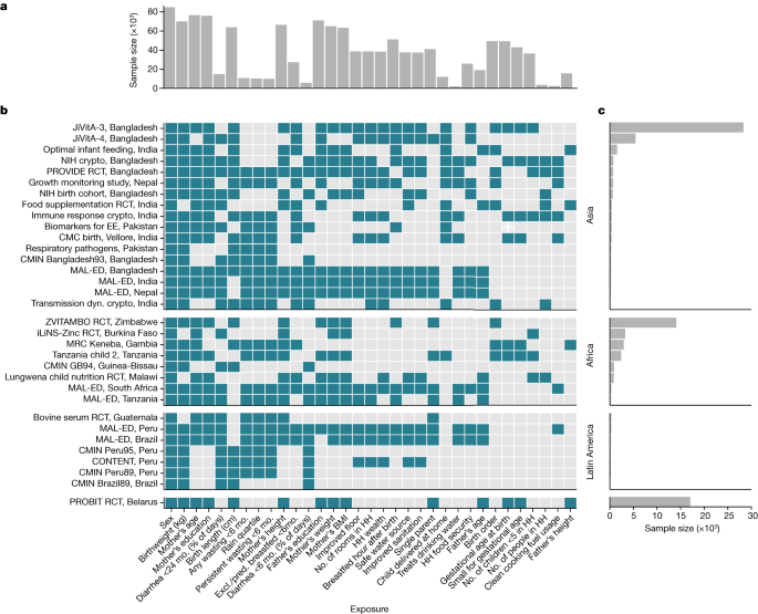
The DHS program website has standard DHS individual recoded files for each country. We used the most recent standard DHS datasets for the individual women’s, household and length and weight datasets from each country, and we estimated age-stratified mean LAZ, WAZ and WLZ from ages 0 to 24 months within each DHS survey, accounting for the complex survey design and sampling weights. See a companion paper for further details on the DHS data cleaning and analysis19. We compared DHS estimates with mean LAZ, WAZ and WLZ by age in the Ki study cohorts with penalized cubic splines with bandwidths chosen using generalized cross-validation63. We did not seasonally adjust DHS measurements.
The child at risk of incident outcomes at birth is the one that was exposed before birth. Therefore, we classified children who were born stunted (or wasted) as incident episodes of stunting (or wasting) when estimating the relationship between household characteristics, paternal characteristics, and child characteristics such as gestational age, sex, birth order and birth location.
We examined covariate missingness by study and assessed the effect of covariate missingness by comparing results with median/mode missingness imputation to a complete-case analysis (Supplementary Note 2). We compared estimates pooled using random-effects models, which are more conservative in the presence of heterogeneity across studies, with estimates pooled using fixed effects (Supplementary Note 3), and we compared adjusted estimates with estimates unadjusted for potential confounders (Supplementary Note 4). The child growth trajectory was plotted for each exposure in the Supplementary Note 5. We re-estimated the attributable differences of exposures on WLZ and LAZ at 24 months, dropping the PROBIT trial, the only European study (Supplementary Note 6). Point estimates and confidence intervals from all age, exposure and growth outcome combinations (as presented in Extended Data Fig. 2) are plotted in Supplementary Note 7.
At 6 months, and after 24 months, the mean difference of exposure on LAZ andWLZ are the same. The measures closest to the age of interest and within a month were used, but not the first one recorded by the child at birth. We took the mean differences for LAZ andWAZ and calculated their weights and lengths.
The estimated prevalence ratios were derived from the comparison levels versus the reference level. Linear regressions were used to estimate mean differences for continuous outcomes.
The Mean Z-scores by continuous age were fit within individual cohorts using a number of squares with the bandwidth chosen to minimize the median Akaike information criterion. We separated the estimates for each exposure category. The pooled curves were used to create a single prediction, offset by the mean of thez-scores at one year.
Optimal individualized intervention impact. Variable importance measure methodology was used to estimate impact of an individualized intervention on exposure63 The optimal intervention on an exposure was determined through estimating individualized treatment regimes, which give an individual-specific rule for the lowest-risk level of exposure based on individuals’ measured covariates. The covariates used to estimate the low-risk level are the same as those used for the adjustment documented in section 6 below. The effect of the individualized intervention is derived from the variable importance measure which is the predicted change in the population mean outcome from the observed outcome if every child were exposed to the optimal level. This differs from the PIE and PAF parameters in that we did not specify the reference level; moreover, the reference level could vary across participants.
To flexibly adjust for potential confounders and reduce the risk of model misspecification, we estimated adjusted prevalence ratios, CIRs, and mean differences using TMLE, a two-stage estimation strategy that incorporates state-of-the-art machine learning algorithms (super learner) while still providing valid statistical inference23,70. There are two plots, one showing the effects on estimates compared to unadjusted estimates and the other showing the strength of unmeasured confounders needed to explain the observed significant associations. The super learner is an ensemble machine learning method that uses cross-validation to select a weighted combination of predictions from a library of algorithms72. The library includes simple means, generalized linear models, LASSO penalised regressions, and generalized additive models. To maximize the AUC for binomial outcomes and to minimize the mean square error for continuous outcomes, the super learner had to be fit. The super learner was able to fit using nine-tenth of the data, and the AUC/MSE was calculated on the remaining one-tenth. Each fold of the data was held out in turn and the cross-validated performance measure was calculated as the average of the performance measures across the ten folds. This approach is practically appealing and robust in finite samples, since this cross-validation procedure uses unseen sample data to measure the estimator’s performance. The super learner is good in the sense that it will perform better as sample size grows. The initial estimator obtained via super learner is subsequently updated to yield an efficient double-robust semi-parametric substitution estimator of the parameter of interest23. Super Learner models with multiple exposures and our estimate of the R2 of models including multiple exposures are within each cohort. We pooled estimates using fixed-effects models.
Analyses used a complete-case approach that only included children with non-missing exposure and outcome measurements. For additional covariates in adjusted analyses, we used the following approach to impute missing covariate values68. Within each cohort, if there was <50% missingness in a covariate, we imputed missing measurements as the median (continuous variables) or mode (categorical variables) among all children, and analyses included an indicator variable for missingness in the adjustment set. Covariates with >50% missingness were excluded from the potential adjustment set. We used children as independent units when calculating the median because children with more frequent measurements were not over-represented.
We did not estimate relative risks between a higher level of exposure and the reference group if there were 5 or fewer cases in either stratum. If there were not a lot of the other exposure and the reference strata, we still estimated the risks between them. For rare outcomes, we only included one covariate for every 10 observations in the sparsest combination of the exposure and outcome, choosing covariates based on ranked deviance ratios.
A pooled incidence method for the outcome prevalence in PAF, PIE and PAFs with unbounded confidence intervals. A comparative study
$${\rm{PAF}}\,95 \% \,{\rm{confidence}}\,{\rm{interval}}=\frac{{\rm{PIE}}\,95 \% \,{\rm{confidence}}\,{\rm{interval}}}{{\rm{Outcome}}\,{\rm{prevalence}}}\times 100$$
The pooled incidence was taken for the outcome prevalence in the above equations. We used this method instead of direct pooling of PAFs because unlike PAFs, PIEs are unbounded with symmetrical confidence intervals.