Extreme weather events in the last ten years: Emergence threshold and birth cohort size in pre-industrial grid cell fractions from sensitivity analysis

The last ten years have been found to be among the ten hottest years recorded in more than two centuries of observations. This anthropogenic climate change is driving not only an increase in the intensity and frequency of extreme weather events, but also changes in the spatial and temporal distribution of such events. For instance, wildfires in Siberia2 and severe floods in Libya have both occurred in the past few years but were historically rare or absent. Extreme weather events are taking place earlier, later or more frequently in the year than in the past, their duration is increasing and historical seasonal patterns are being disrupted — storms, for example, are striking outside their usual seasons. In present-day reality, previously unforeseen events have become part of the process.

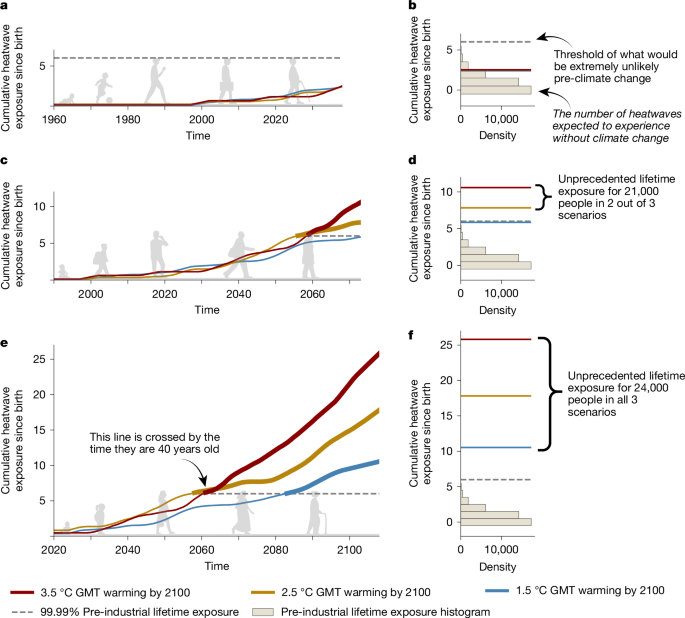
We define an emergence threshold for ULE to extreme events as the 99.99th percentile of our grid-scale samples of pre-industrial lifetime exposure. We went as far as possible with the selection of the percentile, considering the pre-industrial control runs. This choice was based on a sensitivity analysis for different percentile values that showed a levelling off of lifetime exposure for percentiles more extreme than 99.99%. The 99.99th percentile achieved the limit of reliable information that can be found in the empirical distribution. lifetime exposure is assessed for each event and birth year in a pre-industrial climate. We consider the birth cohort to have emerged in this grid cell if this threshold is reached, as the global pool of the same birth cohort and theGMT trajectory of people projected to live ULE. This means that, in some locations, even if the sum of exposed grid cell fractions across a pre-industrial lifetime does not cover the entire grid cell, we still extract the entire birth cohort size associated with that grid cell. We represent the number of people who were emerged in the birth cohort by country, even if the life expectancy is different. The total number of people who have emerged globally is calculated by the total cohort sizes, as well as the birth cohort sizes. ULE does not refer to unprecedented in terms of assets or people exposed but rather in terms of a number of events accumulated across an average person’s lifespan in comparison with what they would face in a pre-industrial climate

To downscale this demographic information to the grid scale, we assume spatially homogeneous cohort representation and life expectancy. Birth cohort size is represented as the number of people of age 0 of a given birth year in a given grid cell. This is estimated by multiplying the absolute population of the birth year (using the annual grid-scale population totals from ISIMIP) by the relative size of the age 0 cohort (using the interpolated 0- to 100-year-old population totals from the Wittgenstein Centre cohort data). Spatial variability in age structure and life expectancy within a country is therefore ignored in this study.

The Inter-Sectoral Impact Model Intercomparison Project: Using GCM input data to calculate extreme event categories of global climate change impacts

Climate change impacts can be projected with a simulation protocol supplied by the Inter-Sectoral Impact Model Intercomparison Project. Impact models represent these sectors are run using atmospheric boundary conditions from a set of biases-adjusted global climate models that were selected based on their availability of daily data. Impact simulations are run for periods before the start of the Industrial Revolution. Representative Concentration Pathways of GCM input are used for future simulations. Impact simulations and GCM input data are used to calculate annual grid-scale fractions of exposure to each extreme event category. We refer to ref. 12 for the full details, but we break down the definitions below.

We know the ranges for the lifetime GDP of a birth year and the single GRDI map, which should align with 2020 population totals. To apply vulnerability indicators to our birth cohort totals on the same grid and year we were born, we need to rank them. For instance, the ranks taken from the lifetime mean GDP of the birth cohort are aligned with population totals of newborns in 2020. Finally, we bin the ranked vulnerability indicators by their associated population totals into five groups of nearly equal population (as it is not possible to achieve perfect bin sizes given the sums of grid-scale population totals). The richest and most deprived are grouped into the quantile ranges. The locations of ULE can be masked by using the quantile range of each vulnerability indicator as a map. With GRDI (Supplementary Fig. 11) and GDP (Supplementary Fig. 12), we compare the lowest and the highest 20% of each indicator by population.