The Second COVID-19 Deaths Reporting Campaign: Focal Points of the WHO and a Circular Letter to WHO Member States
Second, it underlines how much still needs to be done to improve systems for recording deaths. The United Nations wants to find out how many deaths the countries have been able to register as part of the goals. By 2020 154 countries out of 188 that were tracked had death data that was at least 75% complete, according to its latest records. In countries with weak social safety nets, there might be little incentive for people to report deaths. When asked, many people say they didn’t know they needed to. Census-type surveys can fill in some gaps later, but tend to focus on capturing maternal and child mortality. Over half of all deaths aren’t officially counted, according to the UN Children’s charity and a non-profit organization in New York City.
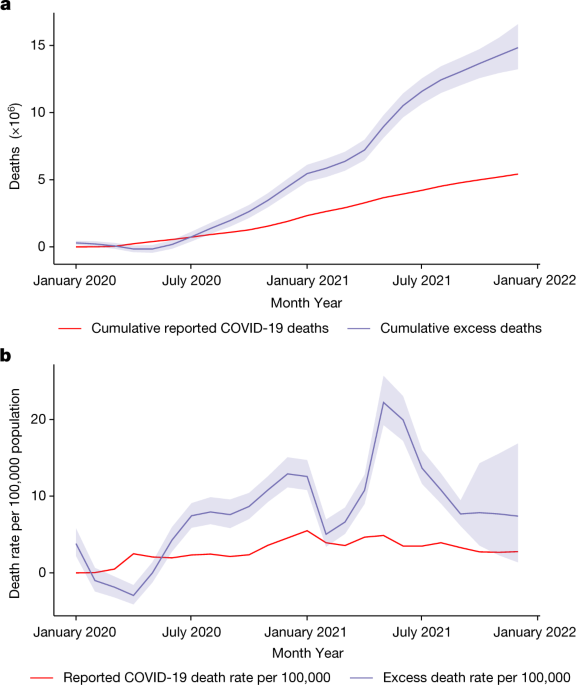
The aim of Msemburi and her associates was to identify the changes in mortality during the Pandemic. Nevertheless, adjusting estimates for these numbers is essential if the goal is to understand COVID-19 fatality better. There are already models available that can adjust for influenza-related avoided mortality10, and new approaches have been proposed for use in the context of the COVID-19 pandemic11. For displaced mortality, partial adjustments can be made by excluding mortality deficits when computing the cumulative number of excess deaths over the months of the observation period. A partial adjustment is made because the deaths that occur during periods of overall deficit remain uncounted.
Improving the processes used to record births and deaths, known as civil registration and vital statistics (CRVS) systems, is crucial to improving public health. Creating better CRVS systems should be part of the treaty prepared by the WHO to strengthen and resilience to future Pandemics. More support should go to ventures that give nations information on how to improve their systems — at present, a hodgepodge of advisory groups are supported by the WHO and by Bloomberg Philanthropies and the Gates Foundation.
In August 2021, a circular letter was sent to all WHO member states to nominate focal points to take part in country consultation. Member states were requested to review the preliminary estimates of excess mortality and submit additional data that may not have been available before. The first round of the country consultation was conducted between October and November of 2021 through WHOs Country Portal, where the draft estimates and methodology for each country were made available to the designated national focal points. Countries that had not nominated a focal point were approached through their respective WHO country office or permanent mission in Geneva, Switzerland.
For all countries and time points we model the expected numbers on the basis of historic data (for most countries, the period 2015–2019 was used for this modelling). We use a negative binomial model that allows for excess-Poisson variation. The annual historic yearly trend is modeled using a model and seasonal variation is modeled using a model. A spline is a flexible approach to modelling that allows departures from a linear association45. A model with two parameters, a mean and scale, accounts for excess-Poisson variation. The mean count for country (c) and in month (t) is modelled as:
WHO Annual Level Data for 2020 and/or 2021: A Model for the Statistical Prevalence, Mortality and Diabetes in Argentine, Indonesia, and Turkey
Data is shared with WHO frequently as part of its standing agreement with member states and specifically provided to WHO in response to a data call for this project.
Additionally, annual level data for 2020 and/or 2021 were obtained from the national statistics offices of China27,28, Grenada29, Saint Kitts and Nevis30, Saint Vincent and the Grenadines31, Sri Lanka32 and Vietnam33.
Where is the relative rate? If it is the case for country and month then it is the case for theta. the mortality is greater than expected, whereas if ({\theta }{c,t} < 1), then for country (c) and at month (t) the mortality is less than expected. We used (G) time-invariant variables, ({Z}{{gc}}) (these are annual values from 2019). The cardiovascular mortality rate and diabetes prevalence rate for the year were indicators of high income and low or middle income. The square root of the reported COVID-19 was computed using the containment variable and B time-varying variables. We build a log- linear model for the rate.
The data for Argentina, India, 40,42, Indonesia and Turkey were obtained from various sources.
Source: https://www.nature.com/articles/s41586-022-05522-2
A Multinomial Model for the National ACM Data in States with Subnational Data and Its Validation using a Poisson Framework
where ({Y}{c,t}) is the realized ACM and ({E}{c,t}) is the ACM that would be expected in the absence of the pandemic. Even countries that have fully observed ACM are affected by the excess because we don’t know the counts that would have happened in the absence of the Pandemic.
We expanded on previous work by constructing a model for the national ACM data in some countries that only subnational data was available. We describe the model in the context of India. We assume that the proportion of deaths in the states with available data remains constant over time, so we use the data from 17 states to estimate the national total. If a state accounts for 10% of deaths in India, one would predict a national death total of 10 deaths in that state. Under the Poisson framework, this proportionality assumption yields a multinomial distribution for the fractions of deaths and we can predict the unknown national totals over the course of the pandemic after fitting the multinomial model.
Both countries with no data and those with subnational data only had model validation done. This included exercises in which we systematically removed all data for each country and took it away for a single month. We used the retained data and evaluated the model performance using metrics such as bias and coverage of prediction intervals. Results for these exercises can be found in the supplementary materials of Knutson et al.15. The model (3) is not used in countries with subnational data.
Source: https://www.nature.com/articles/s41586-022-05522-2
Seasonal variation in association estimation using a time-varying random walk of order 2 and a nonparametric gamma-model
$${{\rm{M}}{\rm{e}}{\rm{a}}{\rm{n}}{\rm{c}}{\rm{o}}{\rm{u}}{\rm{n}}{\rm{t}}}{c,t}=\exp ({{\rm{a}}{\rm{n}}{\rm{n}}{\rm{u}}{\rm{a}}{\rm{l}}{\rm{t}}{\rm{r}}{\rm{e}}{\rm{n}}{\rm{d}}}{c}+{{\rm{s}}{\rm{e}}{\rm{a}}{\rm{s}}{\rm{o}}{\rm{n}}{\rm{a}}{\rm{l}}{\rm{c}}{\rm{o}}{\rm{m}}{\rm{p}}{\rm{o}}{\rm{n}}{\rm{e}}{\rm{n}}{\rm{t}}}_{c,t})$$
For some countries, we only have national historic ACM data. For such countries we model within-year variation using temperature as a surrogate for seasonality. Full details of all modelling steps are given in Knutson et al.15.
where ({\rm{\exp }}\left({\gamma }{g}\right)) and ({\rm{\exp }}\left({\beta }{{bt}}\right)) denote relative rate parameters and ({{\epsilon }}{c,t}\sim {\rm{N}}(0,{{\sigma }}{{\epsilon }}^{2})) are independent error contributions that pick up random variation unexplained by the log-linear regression function. Associations can evolve while the time-varying coefficients are in place. As we desire the evolution to be smooth in time, for these time-varying coefficients ({\beta }_{c,t}) we use a random walk of order 2 (RW2) prior that encourages smooth estimates46. The equation above was conditioned on expected numbers. They are models that give a distribution over plausible values. The uncertainty in the expected predictions is modeled by a gamma distribution, which can be combined with a Poisson model to make a negative binomial model. Knutson et al.15 has full details of evidence of the accuracy of the gamma model.
where the rates ({\theta }_{c,t}) are defined via the log-linear covariate model (3). This allows us to set up the annual counts to correspond to the months of the year.
and ({\text{PS}}_{c,t}\ge -100,) with zero deaths corresponding to –100, negative values corresponding to fewer deaths than expected and larger positive values corresponding to increasing levels of relative excess mortality. We have (textEleft[Y_c,tright]) so that under the model.
For countries whose ACM is unobserved, the rate is modelled via the log-linear form (equation (3)) which gives a specific form to the manner in which we assume the P-score changes as a function of country-specific covariates.
There is an example where we consider the rankings of 27 countries, including the European Union and the United Kingdom, over time.