The Rise of the British-Irish Ice Sheet in the EuIS and its Impact on the Generalized Sloan Digital Skyline (GMSL) Rise
During the last ice age, the British–Irish Ice sheet, the Fennoscandian Ice Sheet and the Svalbard–Barents–kara Ice sheet were the three main sectors of the EuIS. At the start of the Holocene, however, the British–Irish Ice Sheet and the Svalbard–Barents–Kara Ice Sheet were almost gone. The GMSL rise was hampered by the melted water from the Ice Sheet. 46,47,48). Three studies46,47,48 indicate that the EuIS-derived SLE was 2.2 m (2σ range, 1.5–2.9 m) between 11 ka and 10 ka and 3.0 m (2σ range, 2.1–4.3 m) between 11.7 ka and 10 ka (supplementary information49 section 4).
Fox-Kemper, B. et al. The Physical Science Basis: Working Group I contribution to the 6th Assessment Report of the Intergovernmental Panel on Climate Change is related to Climate Change. Ch. 9 (Cambridge Univ. Press, 2023).
Using vibrocores to determine the location of the NAISC and the BRITICE-ChRONO EuIS in the early Holocene
National databases helped identify locations with good prospects of preserving a piece of peat at the maximum depths. In order to determine the exact core location, the surveys were conducted using boomers, sub- bottom profilers and sparkers. The vibrocores were then put in a storage facility at 4 C and cut into metre-long sections. The XRF-scanned vibracores for the 2016 and 2017 cruises were also used.
The background ice-sheet reconstruction was used to define the history of the NAISC. This reconstruction was put together with two other ones for the Eu IS (consistsing of the Norwegian, Barents, Kara Sea, British and North Sea ice sheets). The model was created iteratively using a 1d GIA model to capture the signal in the 18O curve and sea-level data. The BRITICE-CHRONO EuIS model was developed independently of GIA modelling. Using a plastic ice-sheet model71, the spatial and temporal history of the ice sheet was constrained to fit geomorphological and geochronological information (see ref. 14).
The model adopts a spherically symmetrical Maxwell viscoelastic Earth model with three user-defined parameters. To investigate the optimum set of 1D Earth model parameters for each input EuIS reconstruction, we used 1D Earth models with two lithosphere thickness values (71 km and 96 km) combined with upper- and lower-mantle viscosities in the range of 0.1 × 10²¹ Pa s to 1 × 10²¹ Pa s and 1 × 10²¹ Pa s to 50 × 1021 Pa s, respectively, which amounted to 108 models (Extended Data Table 1). Predicting the weighted mean age of each SLIP was used to produce predictions of the model’s temporalresolution from 122 ka to 0 ka.
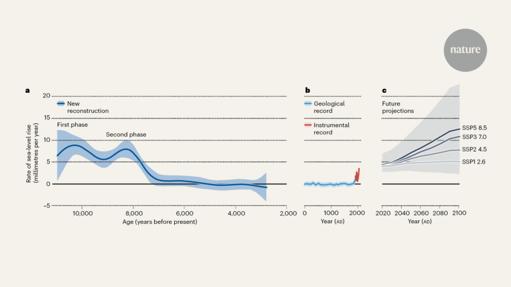
Source: Global sea-level rise in the early Holocene revealed from North Sea peats
Reexamination of the global NAISC-AIS signal from the North Sea region in the early part of the early sea-level rise
$${{\rm{Total\; predicted}}}{{\rm{rsl}}}(\theta ,\varphi ,t)={{\rm{pNAISC}}}{{\rm{rsl}}}(\theta ,\varphi ,t)+{{\rm{pAIS}}}{{\rm{rs}}}(\theta ,\varphi ,t)+{{\rm{pEuIS}}}{{\rm{rsl}}}(\theta ,\varphi ,t)$$
Using equation (2), we calculated both the observed (obsEuISrsl) and predicted (pEuISrsl) EuIS signal by subtracting the predicted contribution from the NAISC (pNAISCrsl) (Extended Data Fig. 7e,g) and the AIS (pAISrsl) (Extended Data Fig. 7d,f) from both the observed (Extended Data Fig. Predicting the total RSL and 7a. 7b,c):
Theta,varphi,t, are all variables that can be applied to the results of the analysis.
This fingerprint ratio, including the 2σ range, was then used to translate the 26.3 m (2σ range, 23.8–28.8 m; 74%) residual SLR in the North Sea region to a global NAISC–AIS signal of 35.5 m (2σ range 27.1–40.0 m; 100%). Adding the EuIS contribution of 2.2 m SLE (2σ range 1.5–2.9 m; see below) after 11 ka results in a total GMSL rise of 37.7 m (2σ range, 29.3–42.2 m) between 11 ka and 3 ka (Fig. 4a). In a next iterative round of running model simulations, Temporal variability of the GMSL fingerprint on the North Sea residual RSL signal can be reexamined by tuning model simulations. This should improve the match between fingerprint-corrected GMSL curves and the geological sea-level observations. The current work was beyond the scope of such an Optimization.
Source: Global sea-level rise in the early Holocene revealed from North Sea peats
Residual RSL Change in HOLSEA Using the Standard Deviation from GIA Models: Application to the EIV-IGP model 37,38
$${\rm{o}}{\rm{b}}{\rm{s}}{\rm{N}}{\rm{A}}{\rm{I}}{\rm{S}}{\rm{C}}+{{\rm{A}}{\rm{I}}{\rm{S}}}{{\rm{r}}{\rm{s}}{\rm{l}}}(\theta ,\varphi ,t)={{\rm{o}}{\rm{b}}{\rm{s}}}{{\rm{r}}{\rm{s}}{\rm{l}}}(\theta ,\varphi ,t)-{\rm{a}}{\rm{v}}{\rm{e}}{\rm{r}}{\rm{a}}{\rm{g}}{\rm{e}}[{{\rm{p}}{\rm{E}}{\rm{u}}{\rm{I}}{\rm{S}}}_{{\rm{r}}{\rm{s}}{\rm{l}}}(\theta ,\varphi ,t)]$$
The uncertainty in obsrsl is taken from the HOLSEA database, whereas for average[pEuIS], the standard deviation calculated from the eight GIA models is used as a measure of uncertainty. From the resulting data series (supplementary information49 section 4), we calculated residual RSL and rates of residual RSL change with the EIV-IGP model37,38 (Extended Data Fig. 9), showing 26.3 m (2σ range, 23.8–28.8 m) of residual SLR for the 11–3 ka period (Fig. 4a).
For the period 11–3 ka, the combined EuIS–NAISC–AIS contribution is then 39.7 m (2σ range, 32.3–46.3 m). It’s a 2 range 35.4–58.6 m for the entire Holocene.
Additional details and references regarding the methods2,8,10,14,16,23,25,32,33,46,47,48,57,58,59,60,61,62,63,64,65,66,86,88,91,94,95,96,97,98,99,100,101,102,103,104,105,106,107,108,109,110,111,112,113,114,115,116,117,118,119,120,121,122,123,124,125,126,127,128,129,130,131,132,133,134,135,136,137,138,139,140,141,142,143,144,145,146,147,148,149,150,151,152,153,154,155,156,157,158,159,160,161,162,163,164,165,166,167,168,169,170,171,172,173,174,175,176,177,178,179 are available in supplementary information49.