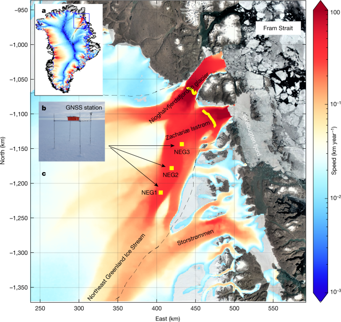
GNSS site-specific observations of the collapse of the floating extension of NG and the transition to sea ice in the Fram Strait
From 2000 to 2021. we use aerial and Landsat 5–10 optical satellite imagery to see the positions of ZI and NG. For ZI, the most notable changes occurred between 2011 and 2013, when a large portion of its floating extension collapsed, resulting in a retreat of 10 km (ref. 53). The retreat was 700 m year1 after the collapse. The main floating tongue has been less frequent since the large sections of it were lost. However, in 2020, the northern section of NG completely collapsed, releasing more than 120 km2 of floating shelf ice into the ocean (Extended Data Fig. 1).
We process the GNSS data using the GIPSY-OASIS software package with high-precision kinematic data processing methods27 and with ambiguity resolution using the orbit and clock products of the Jet Propulsion Laboratory (JPL). The JPL30 developed the GIPSY-OASIS version 6.4. JPL’s finalorbit products include satellite laps, satellite clock parameters and Earth orientation parameters. The phase centre offsets of the satellite antenna are taken into account. The atmospheric delay parameters are modelled using the Vienna Mapping Function 1 (VMF1) with VMF1 grid nominals54. Corrections are applied to remove the solid Earth tide and ocean tidal loading. The amplitudes and phases of the main ocean tidal loading terms are calculated using the Automatic Loading Provider (http://holt.oso.chalmers.se/loading/), which is applied to the FES2014b ocean tide model including correction for the centre of mass motion of the Earth owing to the ocean tides. The site coordinates are computed using the IGS14 frame55. We convert the coordinates into local up, north and east coordinates for each GNSS site monitored at the NEGIS surface. An example of a 15-s solution is shown in Extended Data Fig. The second part of the story is called 2a–c.
The time from the start of each trajectory to the end of sea ice in the Arctic basins was what was defined as the residence time. We calculated an average of residence time of eight pseudo-ice floes that arrived in the Fram Strait at the same time and used it to define the mean residence time of ice floes for each month. The uncertainty of the residence time was decided by the residence time of the pseudo-ice rinks.
An Empirical Semi-Variogram for Ice Surface Elevation Changes and Elastic Uplift of the Bedrock at NEG1 and NEG2
The flow acceleration, which compensates for the downhill movement of the GNSS stations, have correction rates of 0.06 0.18 m year2 at NEG1, and 0.29 0.29 m year2 at NEG2.
Extended Data Fig. 4c shows the same information as Extended Data Fig. 4b but for the point P2, which is located at about 1,078 m elevation. Here the amplitude of the annual signal is 0.16 ± 0.08 m.
The data is extended. 7 shows annual elevation change rates from April to April for the period from April 2011 to April 2021 that are corrected for GIA and elastic uplift. In the lower panels there are uncertainties associated with the annual elevation change rates.
The annual elevation change rates that are observed from NASA as well as ICESat-2 are combined to calculate a regular grid of 1 1 km. The interpolation is performed using the ordinary kriging method59,60. We use the observed annual elevation change rates to estimate an empirical semi-variogram. We fit a model variogram to the empirical semi-variogram to take the spatial correlation of elevation change rates into account. For each grid point, we estimate the elevation change rate dhi,krig and the associated error σi,krig.
An example of elevation changes at the overlap points can be seen in the Extended Data panel. The largest elevation change is observed near the glacier margin.
We modify the ice surface elevations for bedrock movement as a result of the long-term past ice changes. We use the GNET-GIA model61 to correct for GIA. For each grid point, we estimate the GIA uplift rate dhGIA and the associated uncertainty σGIA. We correct for the elastic uplift of the bedrock by convolving ice loss estimates (from CryoSat-2, ATM and ICESat-2) with the Green’s functions derived by Wang et al.62 for the elastic Earth model iasp91 with a refined crustal structure taken from CRUST 2.0. For each grid point, we have an estimate of what the elastic rate is going to be. The elevation change rate for each grid point.
There is extended data in this fig. The models show the change in the ice mass over the course of a few years. For each friction law, we model the mass change using RCP4.5 and RCP8.5, respectively. NorESM1 was used for all models. For comparison, we include results from ref. 8 that were calculated using the Budd friction law (linear viscous). According to the data, the uncertainty of the mass change from the regularized Coulomb friction law is only about one-third of the observed mass change. The Budd friction law with exponents of 1/5 or 1/6 slightly overestimates the mass change from 2007 to 2021. However, we note that, by 2100, the mass loss from the Budd friction law with exponents of 1/5 or 1/6 is almost the same as that from the regularized Coulomb friction law. The retreat from the beginning of 2007, using NorESM1, RCP4.5 and regularized Coulomb friction law, is shown in Supplementary Video 1.
In Extended Data Fig. 9, we consider models that are able to reproduce deep inland acceleration. Therefore, the choice of friction laws is reduced to the regularized Coulomb friction law and the Budd friction law with exponents of 1/5 and 1/6, as all the other models were unable to generate deep inland acceleration.
Sea ice draft measurement from upward looking sonars in the Fram Strait: data gaps and sensitivity of the draft to underwater fraction
Sea ice draft data were obtained from upward looking sonar (ULS) moored in the East Greenland Current in the western Fram Strait. There are short temporal gaps in the last three decades of the dataset. Four ULSs were zonally aligned at approximately 79° N from 3° W to 6.5° W (Fig. 1a). The latitude of the mooring array changed from 79° N to 78.8° N in 2001. The moorings have names like 3 W (F11),4 W (F12),5 W (F13) and 6.5 W (F14). In the last three decades of measurement, there are three main temporal data gaps. The number of ULSs varied from time to time but they were still in operation. The ULS measures the travel time of the sound reflected at the bottom of the floating sea ice, from which we calculate the ice draft, the underwater fraction of sea ice54. The raw data were processed to ice draft using procedures described in earlier literature55,56. The accuracy of each draft measurement ranges from 0.1 m (ice profiling sonars (IPS) deployed after 2006) to 0.2 m (ES300 instruments before 2006), while the uncertainty of each individual measurement is not subject to bias errors and the summary error statistics of monthly values are less than 0.1 m57.
$$f({X}{m})=\frac{1}{\sqrt{2{\rm{\pi }}\mathop{\sigma }\limits^{ \acute{} }{(m)}^{2}}{X}{m}}\exp \left(\frac{-{({\rm{l}}{\rm{n}}({X}_{m}/\mathop{X}\limits^{ \acute{} }(m)))}^{2}}{2\mathop{\sigma }\limits^{ \acute{} }{(m)}^{2}}\right)$$
thinner ice has a better chance of being ridged and/or rafted if a dynamic event occurs than thicker ice. To implement this feature, α is given by a function of ice thickness: the areal probability is inversely proportional to the stochastic ice thickness Xi:
where (\acute{X}(m)={e}^{\nu m}) and (\acute{\sigma }(m)=\sigma {m}^{1/2}) and ν and σ2 are the mean and variance of the population distribution of ln am (including X0), respectively67.
$${a}{i}=\left{\begin{array}{cc}1+b{r}{i} & {\rm{w}}{\rm{i}}{\rm{t}}{\rm{h}}\,{\alpha }{i}({\rm{ \% }})\,{\rm{p}}{\rm{r}}{\rm{o}}{\rm{b}}{\rm{a}}{\rm{b}}{\rm{i}}{\rm{l}}{\rm{i}}{\rm{t}}{\rm{y}}\ 1 & {\rm{w}}{\rm{i}}{\rm{t}}{\rm{h}}\,1-{\alpha }{i}({\rm{ \% }})\,{\rm{p}}{\rm{r}}{\rm{o}}{\rm{b}}{\rm{a}}{\rm{b}}{\rm{i}}{\rm{l}}{\rm{i}}{\rm{t}}{\rm{y}}\end{array}\right.$$
Source: https://www.nature.com/articles/s41586-022-05686-x
On the number of dynamic events for sea ice formation and ridging: The case of the Arctic cyclones in the summer and winter
Another parameter necessary for the model is the number of dynamic events, m, that is, external forcing that could cause mechanical fracturing of sea ice and consequent ridging and/or rafting. We used the number of Arctic cyclones that passes over the ice pack as a first-order indicator of the number of dynamic events. Typically 90 to130 cyclones per year occur in the tropics, but most occur in the summer and winter. A typical size of an Arctic cyclone is approximately 3 × 10⁶ km2 (mean radius of approximately 103 km)71, which covers approximately one third of the ice-covered area of the Arctic Ocean. We assumed that the ice pack in the North experiences approximately 40 dynamic events per year, which means one-third of all storms hit at a certain location. The average residence time of sea ice in thearctic is 2–6 years.
where c is the thermodynamic ice growth coefficient. This term comes from a simplified thermodynamic process without thermal inertia of sea ice and heat flux from the ocean72: